Cable Diameter Calculation Guide: Formulas, Charts & Tables
2026-04-07
In modern electrical and telecommunications engineering, accurate cable diameter determination stands as a foundational requirement for system reliability, safety, and performance. From industrial power distribution to high-speed data networks, selecting the correct diameter affects current-carrying capacity, voltage drop, heat dissipation, mechanical installation, and long-term durability.
Cable diameter is a fundamental parameter in electrical engineering and industrial design. It directly influences current-carrying capacity, voltage drop, thermal performance, and mechanical flexibility. In real-world export-oriented manufacturing—especially for transformers, power distribution systems, and industrial automation—incorrect cable diameter selection can lead to overheating, insulation failure, or even system downtime.
Understanding Cable Diameter vs. Cross-Sectional Area
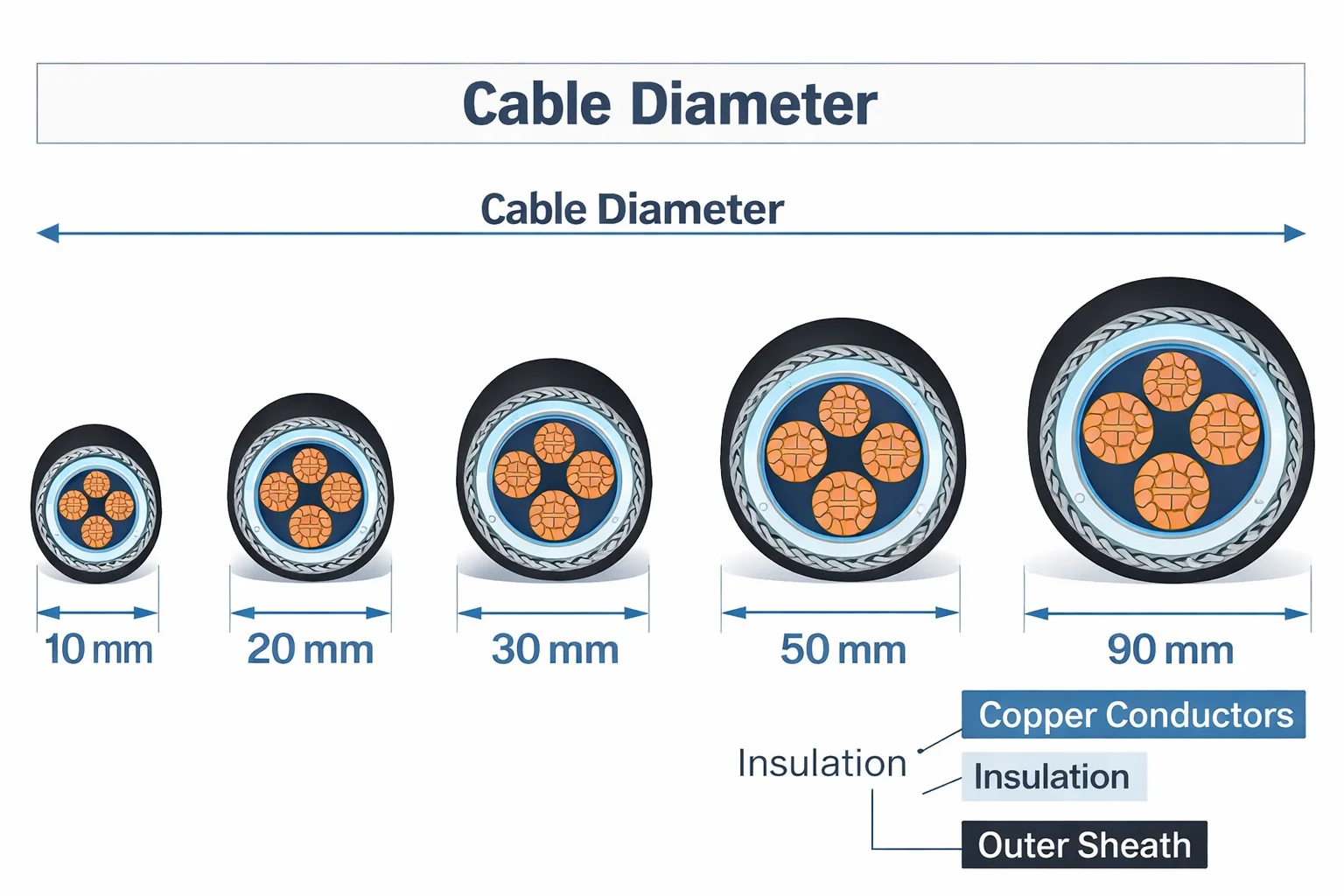
Cable diameter refers to the overall outer measurement of a conductor or finished cable, while cross-sectional area (typically in mm² or circular mils) defines the conductive portion responsible for current flow. These two metrics connect through basic geometry but differ significantly in application. The conductor itself follows the circle area formula:
A = π × (d/2)² = (π × d²)/4
where A is the cross-sectional area in mm² and d is the conductor diameter in mm. Rearranged to solve for diameter:
d = 2 × √(A / π) ≈ 1.1284 × √A
This relationship proves critical when converting between AWG sizes and metric equivalents or when verifying manufacturer specifications. However, the finished cable outer diameter includes insulation, shielding, and jacketing, which can increase the total measurement by 50–200% depending on the cable type. In field work, always distinguish bare conductor diameter from overall cable diameter to avoid conduit fill violations or bending radius issues.
Practically, undersizing the diameter leads to overheating and fire hazards, while oversizing increases material costs and installation difficulty. Engineers must balance ampacity tables, voltage drop limits (typically ≤3–5% for power circuits), and environmental factors such as ambient temperature and bundling.
Key Formulas for Cable Diameter Calculation
Several core formulas support daily cable diameter calculation:
- Single Conductor Diameter from Area d (mm) = √(4 × A / π). This applies directly to solid conductors. For example, a 10 mm² copper conductor yields d ≈ 3.57 mm.
- Stranded Conductor Approximation. For stranded wires, the effective diameter accounts for the stranding lay factors. A common practical multiplier for the overall conductor bundle is approximately 1.15–1.25 times the equivalent solid diameter, depending on strand count and lay length.
- Wire Bundle Diameter When multiple insulated wires form a bundle (common in control panels or harnesses), use: Bundle Diameter ≈ k × √(n) × single wire diameter where n is the number of wires and k is a packing factor (typically 1.2 for random lay, up to 1.8–2.0 for tight bundles). More precise methods sum individual cross-sectional areas first, then apply the circle diameter formula to the total area. In practice, add a 10–20% margin for irregular packing and movement.
- Voltage Drop Influenced Sizing Required area A (mm²) = (2 × L × I × ρ) / (ΔU × cosφ) for single-phase, where L is length (m), I is current (A), ρ is resistivity (0.0178 Ω·mm²/m for copper at 20°C, 0.0282 for aluminum), and ΔU is allowable voltage drop. Convert the resulting area to diameter using the formula above. This calculation often drives final selection in long-run industrial installations.
These formulas provide the scientific backbone, but field experience shows that real cables deviate slightly due to manufacturing tolerances (±5–10% on diameter) and temperature effects on resistivity.
1. AWG Wire Conductor Diameter Chart (Copper Solid Conductor)
This table focuses on the fundamentals of cable diameter calculation and is applicable to power wires and cables.
|
AWG Size |
Conductor Diameter (mm) |
Cross-Sectional Area (mm²) |
Typical Applications |
Notes for Field Use |
|
22 AWG |
0.64 |
0.326 |
Signal, instrumentation, low-current control |
Flexible stranded version slightly larger (~0.7-0.8 mm) |
|
12 AWG |
2.05 |
3.31 |
Lighting, general outlets (15-20A) |
Common in residential/commercial wiring |
|
8 AWG |
3.26 |
8.37 |
Subfeeds, higher power circuits |
Good balance of ampacity and flexibility |
|
6 AWG |
4.11 |
13.3 |
50-75A circuits, motors |
6 awg cable diameter critical for voltage drop |
|
4 AWG |
5.19 |
21.1 |
Heavy-duty branch circuits |
4 awg cable diameter often used in industrial panels |
|
4/0 (0000) |
11.68 |
107 |
Main feeders, high-ampacity runs |
4 0 cable diameter requires large conduits |
Note: The above figures are for bare solid conductors. Stranded conductors have an effective diameter that is approximately 5-15% larger. Copper & Aluminum: Aluminum conductors have higher resistivity, requiring a larger cross-sectional area (approximately 1.6 times) for the same current, thus increasing the cable diameter. Always refer to the latest NEC/IEC ampacity table and consider temperature derating.
AWG System and Practical Diameter Charts for Copper & Aluminum
The American Wire Gauge (AWG) system remains the global standard for many exported wires and cables, especially in North American and international markets. Larger AWG numbers indicate smaller diameters. Here are typical bare conductor values for common sizes (solid conductor approximations; stranded versions are marginally larger in overall diameter):
- 22 AWG cable diameter: ~0.64 mm (area 0.326 mm²) – ideal for low-current signal and instrumentation wiring.
- 12 AWG cable diameter: ~2.05 mm (area 3.31 mm²) – common for general lighting and outlet circuits (up to ~20–25A depending on insulation).
- 8 AWG cable diameter: ~3.26 mm (area 8.37 mm²) – suitable for higher power subfeeds.
- 6 AWG cable diameter: ~4.11 mm (area 13.3 mm²) – frequently used for 50–75A circuits.
- 4 AWG cable diameter: ~5.19 mm (area 21.1 mm²) – heavy-duty branch circuits.
- 4/0 cable diameter (also called 0000 or 4 0): ~11.68 mm (area 107 mm²) – large power feeders carrying hundreds of amps.
For Copper & Aluminum comparisons, aluminum requires approximately 1.6 times larger cross-section than copper for equivalent resistance due to higher resistivity. Thus, a 4 AWG copper (≈21 mm²) roughly equates to a 2 AWG aluminum in performance, but the physical diameter increases accordingly. Always consult dual-rated ampacity tables, as aluminum derates more aggressively for heat.
Stranded conductors, preferred for flexibility in export equipment, maintain the same nominal area but present a slightly larger effective diameter. In practice, measure or request manufacturer data sheets for the exact overall cable diameter, including insulation.
Coaxial Cable Diameter Considerations
Coaxial cable diameter directly impacts impedance (typically 50Ω or 75Ω), attenuation, and power handling. The characteristic impedance formula is:
Z₀ = (138 / √ε) × log₁₀(D/d)
where D is the inner diameter of the shield and d is the conductor diameter, with ε as the dielectric constant. Common RG6 coaxial cable diameter ranges 6.5–7.0 mm overall, while RG11 is thicker for lower loss over distance. In field installations, a larger coaxial cable diameter reduces signal attenuation at high frequencies but complicates routing. Always match connector dimensions precisely to the cable's outer and dielectric diameters to maintain performance in broadcast or CCTV systems.
Data and Network Cables: Cat 6 Cable Diameter
Cat 6 cable diameter typically measures 5.5–6.8 mm overall, larger than Cat 5e due to thicker 23 AWG conductors and internal separators that reduce crosstalk. This increased diameter affects conduit fill calculations—engineers must limit fill to 40% for easy pulling. In dense data center deployments, the larger cat 6 cable diameter improves performance up to 10 Gbps over 100m but requires careful pathway planning. Shielded versions (F/UTP or S/FTP) add further to the diameter, often reaching 7–8 mm.
1. Typical Overall Cable Outer Diameter (with Insulation) – Copper Power Cables
This table reflects the actual cable outer diameter in the installation (taking common insulation such as THHN/XLPE as an example; the values are approximate and may vary depending on the manufacturer).
|
AWG Size |
Approx. Overall Diameter (mm) |
Insulation Type Example |
Max Recommended Current (Copper, 75°C) |
Key Consideration |
|
22 AWG |
1.8 – 2.5 |
PVC/PE |
3 – 7 A |
Signal integrity |
|
12 AWG |
3.8 – 4.5 |
THHN |
20 – 25 A |
Conduit fill limit |
|
8 AWG |
5.5 – 6.5 |
THHN/XLPE |
40 – 55 A |
Heat dissipation in bundles |
|
6 AWG |
6.5 – 8.0 |
THHN/XLPE |
55 – 75 A |
6 awg cable diameter for voltage drop calc |
|
4 AWG |
8.0 – 9.5 |
XLPE |
70 – 95 A |
Mechanical strength |
|
4/0 |
15 – 18 |
XLPE/PVC |
200+ A |
Large bending radius required |
Note: Insulation thickness will significantly increase cable diameter. Aluminum cables of the same specifications typically have a larger outer diameter. Field recommendation: Measure a sample cable and allow a 10-15% margin for bundle or environmental factors.
Fiber Optic Cable Diameter
Fiber optic cable diameter varies widely by construction. Individual fibers have a standard 125 μm cladding with 250 μm coating, but finished cables range from 2–3 mm for simplex patch cords to 10–20 mm or more for high-fiber-count armored outdoor cables. Loose-tube designs accommodate thermal expansion, while tight-buffered versions prioritize flexibility. When calculating pathway capacity, treat fiber optic cable diameter similarly to copper but factor in minimum bend radius (typically 10–20× outer diameter) to prevent macrobending loss. In international export projects, hybrid copper-fiber cables demand integrated diameter planning for shared conduits.
1. Special Cable Types Diameter Comparison Chart
|
Cable Type |
Typical Overall Diameter (mm) |
Common Variants |
Key Performance Impact |
Practical Installation Tips |
|
Coaxial Cable (RG58) |
4.8 – 5.0 |
50Ω |
Higher frequency → larger diameter for lower loss |
Match the connector precisely |
|
Coaxial Cable (RG6) |
6.5 – 7.0 |
75Ω (broadband/TV) |
Coaxial cable diameter affects attenuation |
Outdoor: add UV jacket |
|
Coaxial Cable (RG11) |
9.5 – 10.5 |
75Ω (long runs) |
Lower loss over distance |
Heavier, harder to bend |
|
Cat 6 UTP |
5.5 – 6.5 |
23-24 AWG conductors |
Cat 6 cable diameter is larger than Cat5e |
Max 40% conduit fill |
|
Cat 6 F/UTP (Shielded) |
6.5 – 8.0 |
Foil shield |
Better EMI protection, slightly larger diameter |
Grounding critical |
|
Fiber Optic Patch Cord |
1.6 – 3.0 |
Simplex/Duplex (2.0mm common) |
Fiber optic cable diameter is small & flexible |
Bend radius ≥10× OD |
|
Multi-Fiber Outdoor Cable |
8 – 20+ |
12-24 fibers, loose tube |
Armored versions thicker |
Pulling the tension limit |
Note: Coaxial cable diameter directly affects impedance matching (Z₀ formula). Cat 6 cable diameter affects path planning in dense cabling in data centers. Fiber optic cable diameter must strictly adhere to the minimum bending radius to prevent signal loss. For hybrid cabling, calculate the overall fill ratio uniformly.
Practical Cable Sizing from the Field Perspective
In real projects, begin with load analysis: calculate maximum current, apply derating for temperature, bunding, and ambient conditions, then select the smallest diameter that satisfies ampacity and voltage drop. Next, verify mechanical aspects—conduit fill (NEC or IEC limits), bending radius, and pulling tension. For Copper & Aluminum, copper offers better conductivity and corrosion resistance in humid environments, while aluminum reduces weight and cost for long overhead runs, albeit with a larger required cable diameter.
Bundle calculations deserve special attention in control cabinets. Overly tight bundles reduce heat dissipation, necessitating larger individual diameters or derating. Modern design software helps, but manual verification using the area summation method remains essential for accuracy.
Temperature also influences effective diameter indirectly through expansion and resistance changes. Copper resistivity rises ~0.4% per °C, potentially requiring upsizing in hot environments.
Charts and Quick Reference Tables
While exact values depend on stranding and insulation, standard references show:
- Smaller gauges (22–12 AWG) suit signal and branch circuits.
- Mid-range (8–4 AWG) handle sub-panels and motors.
- Large sizes (4/0 and above) serve main feeders.
Always cross-reference with current standards (NEC, IEC 60364) and manufacturer datasheets, as insulation types (THHN, XLPE, PVC) add varying thicknesses to the final cable diameter.
1. Copper vs Aluminum Quick Comparison (Same Ampacity)
|
Parameter |
Copper Example (6 AWG) |
Aluminum Equivalent |
Diameter Impact |
Field Advantage |
|
Cross-Section (mm²) |
13.3 |
~21 (approx. 4 AWG) |
Aluminum larger |
Copper: smaller diameter, easier install |
|
Conductor Diameter (mm) |
4.11 |
~5.2+ |
+20-30% |
Aluminum: lighter, lower cost for long runs |
|
Typical Overall OD (mm) |
6.5-8.0 |
8.0-10.0 |
Noticeable |
Copper is better in corrosive/humid environments |
Note: Aluminum requires a larger cable diameter to compensate for resistivity, but it has a significant weight advantage. In actual projects, the selection should be based on a careful consideration of voltage drop and cost.
Conclusion: Best Practices for Accurate Cable Diameter Selection
Effective cable diameter calculation combines geometric formulas, material properties of Copper & Aluminum, and application-specific factors for coaxial cable diameter, cat 6 cable diameter, fiber optic cable diameter, and power wires. From initial load calculations through final installation verification, a systematic approach prevents costly rework and ensures compliance in international markets.
Engineers should maintain a personal reference library of AWG/mm² charts, voltage drop calculators, and bundling factors. In practice, measure sample cables during prototyping and apply conservative margins. This disciplined methodology delivers safe, efficient, and future-proof wires and cables systems that perform reliably under real-world conditions.
Related Articles

Related Products
1500kVA Oil Immersed Transformer
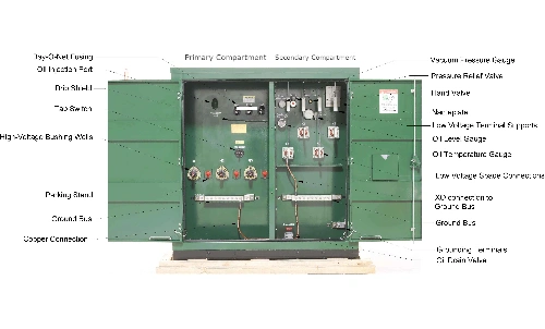
NPC ELECTRIC's 1500kVA oil-immersed transformer adopts advanced technology, complies with international IEC, ANSI, and other standards, and has efficient and stable power conversion capabilities. It uses oil-immersed cooling technology, has excellent heat dissipation performance and durability, and ensures long-term stable operation of the equipment in harsh environments. Primary voltages range from 2.4kV to 34.5kV (common: 34.5kV, 24.94kV, 13.8kV, 13.2kV, 12.47kV, 4.16kV) in delta or grounded wye configurations with BIL up to 200kV.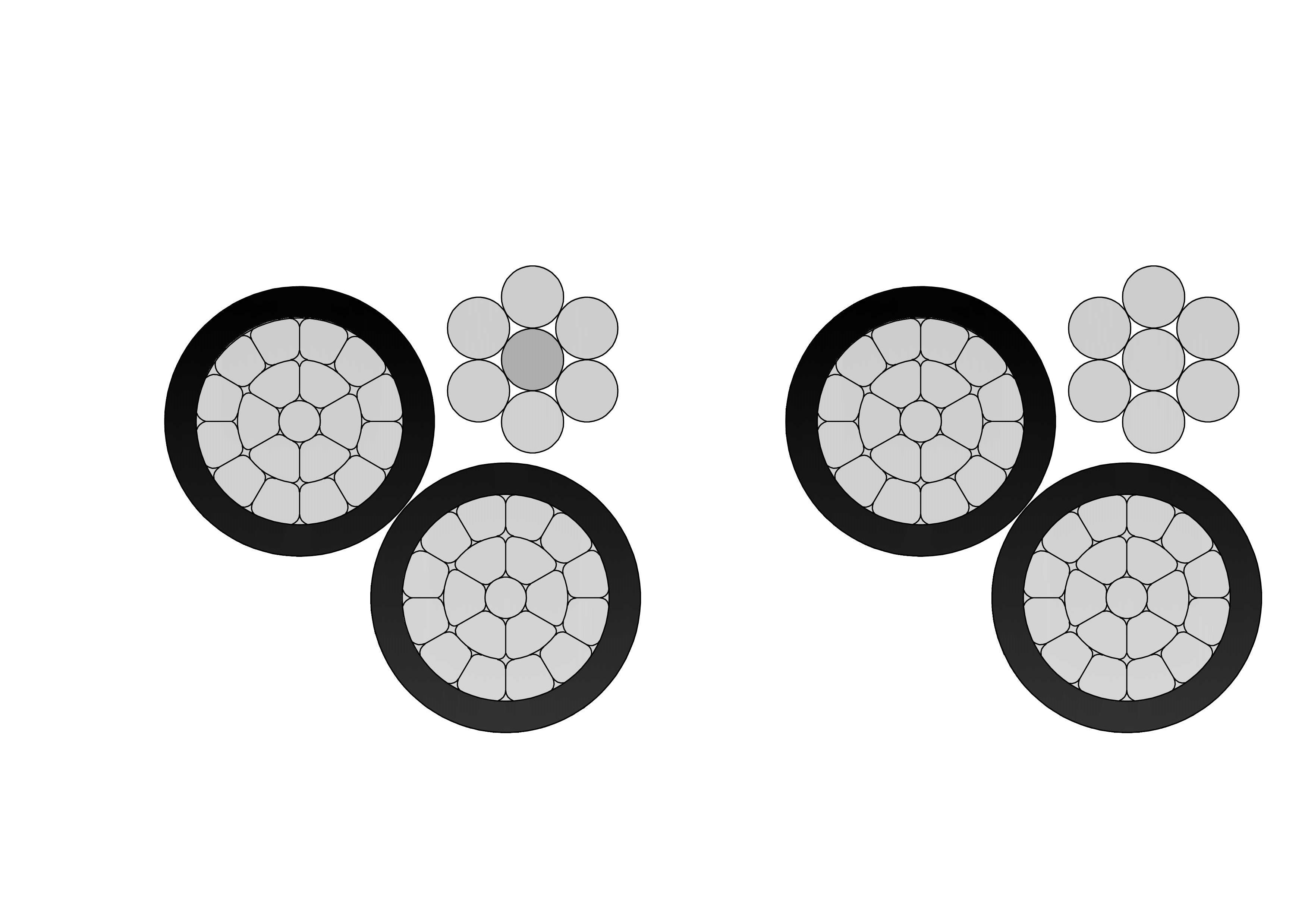
6 Minex Aluminum Conductor Triplex Overhead Service Drop Cable
The 6 Minex Aluminum Conductor Triplex Overhead Service Drop Cable is engineered for reliable overhead power distribution from utility lines to service entrances. The cable structure consists of two insulated aluminum phase conductors twisted around a reinforced neutral messenger, delivering stable electrical performance and strong mechanical support. Manufactured from high-purity aluminum and weather-resistant insulation materials, the 6 Minex Aluminum Conductor Triplex Overhead Service Drop Cable offers excellent conductivity, low weight, and ease of installation. The insulation system is designed to withstand UV radiation, moisture, temperature fluctuations, and environmental aging, ensuring dependable long-term outdoor performance. A comprehensive quality control system is applied throughout production. The 6 Minex Aluminum Conductor Triplex Overhead Service Drop Cable undergoes systematic raw material testing, continuous process inspection, and rigorous finished product testing. Each stage follows standardized procedures to ensure compliance with international standards and utility specifications. This cable is an ideal solution for residential, commercial, and light industrial overhead service drop applications requiring safety, durability, and consistent quality.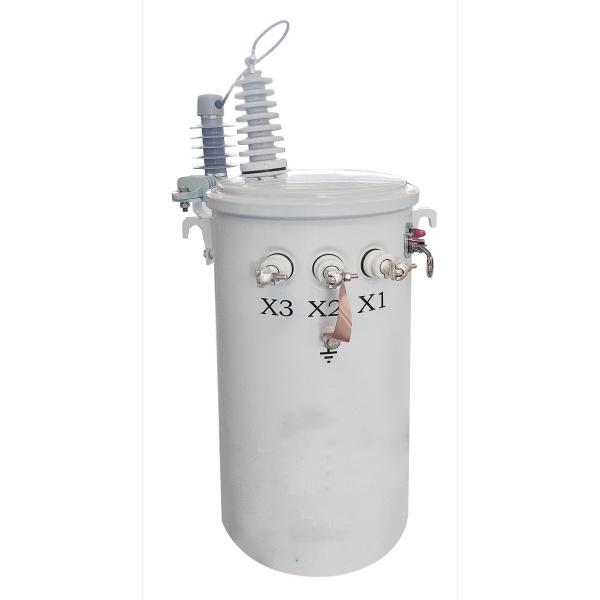
100kVA Completely self-protected(CSP) Single Phase Pole Mounted Transformer
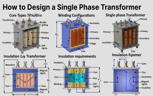
100kVA CSP Single Phase Pole Mounted Transformer is a highly efficient and reliable solution designed for single-phase power distribution in residential, commercial, and light industrial applications. It features integrated self-protection systems, including overload, short-circuit, and over-voltage protection, ensuring automatic disconnection in the event of faults to safeguard both the transformer and connected equipment. With its pole-mounted design, it offers space-saving installation and is suitable for both urban and rural environments. This transformer delivers high operational efficiency with minimal energy loss and is built to withstand harsh weather conditions, ensuring long-lasting and reliable performance. It is the ideal choice for providing safe and stable single-phase power in diverse applications.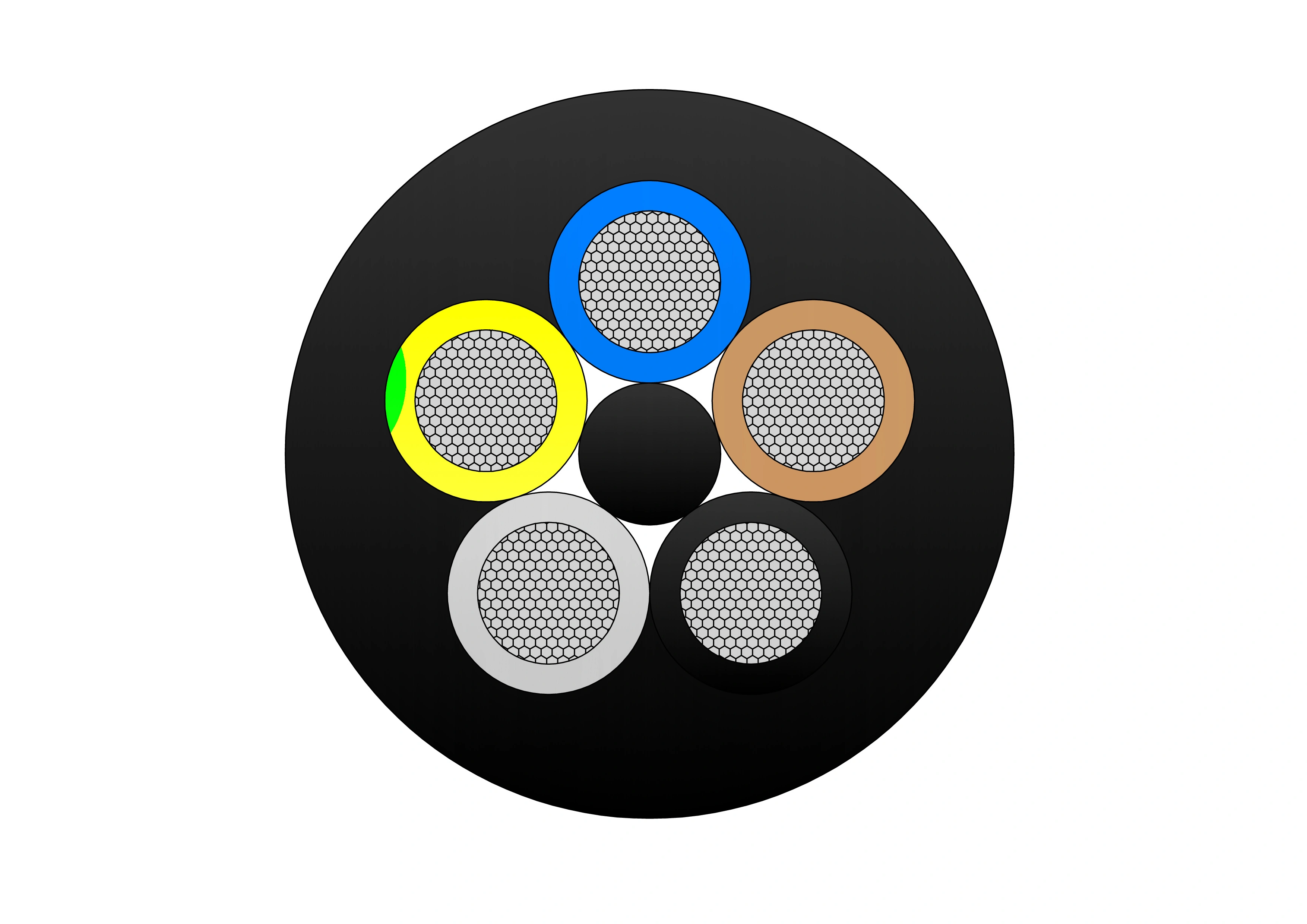
(N)TSCGECECWOU 3.6/6kV and 6/10kV ZH Cable
The (N)TSCGECECWOU is a flexible medium voltage reeling and trailing cable manufactured in compliance with DIN VDE 0250 standards. Designed for demanding mining, tunneling, and heavy industrial applications, it offers exceptional mechanical strength, flexibility, fire safety, and electromagnetic compatibility (EMC). The cable features EPR insulation, low smoke zero halogen (LSZH) inner sheath, halogen-free polyurethane (PUR) outer sheath, and a copper wire braid with concentric conductor for enhanced shielding and durability. Its design ensures reliable performance in environments requiring fire safety, oil resistance, and high torsional strength.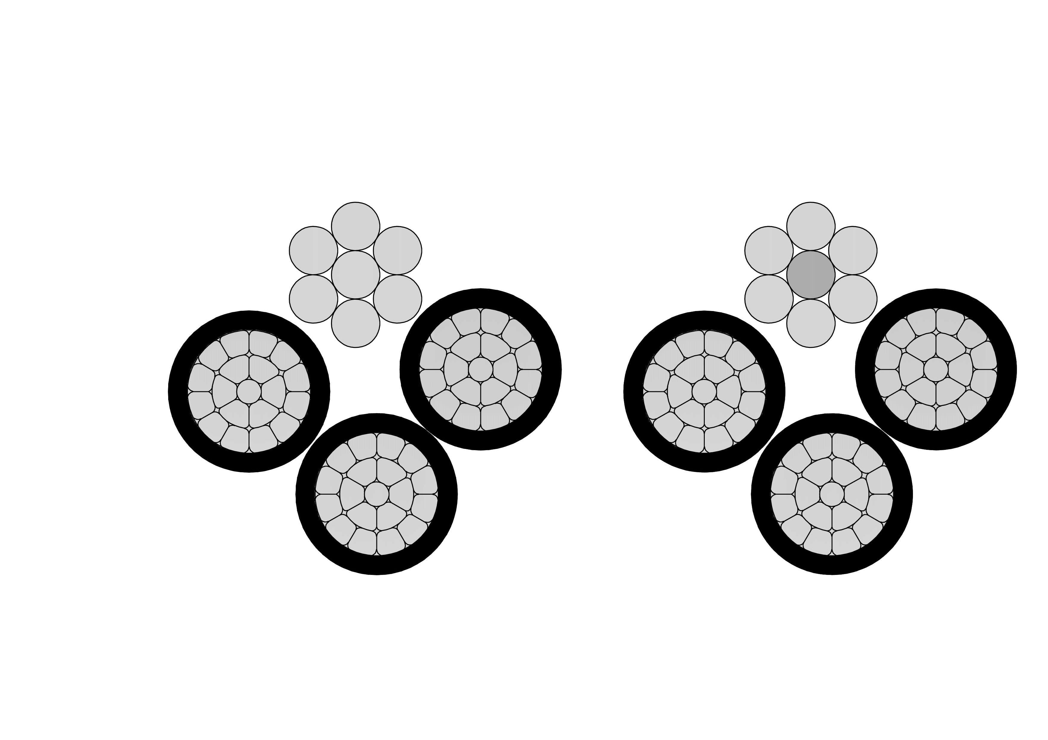
Quadruplex Service Drop Cable
NPC Electric Quadruplex Service Drop Cable offers efficient overhead three-phase service with neutral support. Comprising three-phase conductors (aluminum) insulated with XLPE or PE and helically twisted around a strong neutral messenger (ACSR, AAC, or covered aluminum), it meets ASTM, ICEA, and international standards. The messenger provides full self-support, allowing longer spans and reduced infrastructure costs. Premium insulation resists sunlight, moisture, and mechanical abrasion for decades of outdoor service. Lightweight and flexible, it simplifies installation with low sag. The Quadruplex Service Drop Cable ensures minimal losses, high mechanical endurance, and excellent weather performance up to 600V. Flame-retardant options enhance safety. Perfect for reliable power delivery in urban developments, commercial areas, street lighting, and temporary sites requiring safe, cost-effective aerial bundled solutions.
200kVA Single Phase Pole Mounted Transformer
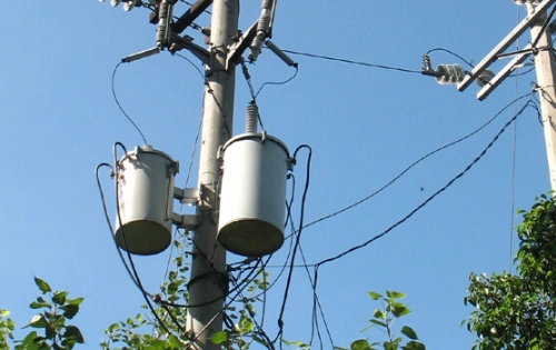
NPC ELECTRIC'S 200kVA single phase pole mounted transformer delivers exceptional reliability for demanding overhead power systems. It efficiently converts primary voltages like 11kV or 22kV to secondary levels such as 220V or 400V, supporting heavier loads in diverse environments. Constructed with low-loss grain-oriented steel cores and high-grade aluminum conductors, it achieves superior energy efficiency and reduced operational costs. Meeting ANSI/IEEE C57 standards, the weatherproof enclosure ensures protection against elements, with a 55°C temperature rise and ONAF cooling for enhanced performance. Essential safety integrations include overload fuses and oil level gauges, making it suitable for utilities aiming for minimal downtime. This transformer excels in providing stable power with low harmonic distortion, ideal for modern grid upgrades.
250kVA Three Phase Pad Mounted Transformer
The 250kVA Three Phase Pad Mounted Transformer is a compact, liquid-immersed, self-cooled (ONAN) distribution transformer optimized for efficient, underground power delivery in residential, light commercial, and small industrial applications. Fully compliant with IEEE C57.12.34, ANSI C57.12.00, DOE 2016 efficiency standards, and UL-listed, this compartmental-type unit features dead-front 200A high-voltage bushing wells (loadbreak inserts), radial or loop feed options, and a sealed tank using non-PCB mineral oil or FR3 natural ester fluid for improved fire safety and environmental performance.
22kV Dry Type Transformer Cast Resin Three Phase Distribution Transformer
22kV Dry Type Transformer Cast Resin Three Phase Distribution Transformer, a premium oil-free solution engineered for safe, reliable medium-voltage power distribution in indoor environments. This three-phase cast resin transformer features fully vacuum-impregnated epoxy resin windings with high-conductivity copper conductors and premium low-loss grain-oriented silicon steel cores, achieving superior energy efficiency (typically 98.5%+), significantly reduced no-load and load losses, and excellent partial discharge performance (<10pC). The advanced cast resin encapsulation provides outstanding moisture resistance, self-extinguishing fire safety (F1 class), robust short-circuit withstand capability, and completely maintenance-free operation. Natural air (AN) cooling with optional forced air (AF) upgrades supports high overload capacity, while optimized core clamping, vibration-dampening mounts, and noise-reduction design deliver low acoustic levels suitable for urban or sensitive installations.
25kVA Conventional Type Single Phase Pole Mounted Transformer
NPC ELECTRIC'S 25kVA Conventional Type Single Phase pole Mounted transformer are designed for servicing residential overhead distribution loads. They are also suitable for light commercial loads, industrial lighting and diversified power applications. These transformers are designed for the application conditions normally encountered on electric utility power distribution systems. Types CSP, CP, SP and S are all available. ISO 9001: 2008 Certified. Typical specifications include mineral oil insulation (ONAN cooling), aluminum or copper windings, primary voltages 2.4 kV–34.5 kV grounded wye or delta (most common: 7200/12470GrdY, 7620/13200GrdY, 12470GrdY/7200, 24940GrdY/14400, 34500GrdY/19920), secondary 120/240 V or 240/120 V split-phase, BIL ratings 95–150 kV HV / 30 kV LV, impedance typically 2.0–4.0%, ±2×2.5% or 5-position tap changer, conventional or completely self-protected (CSP) versions with internal primary fuses, external weak-link cutout, lightning arresters, pressure relief device, oil sight gauge, and standard ANSI 70 gray tank finish. Efficiency usually reaches 98.90%–99.10%+, with low sound level and corrosion-resistant design for long outdoor service life.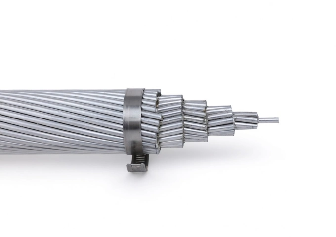
477 MCM Cosmos AAC Cable
The 477 MCM Cosmos AAC Cable represents premium All Aluminum Conductor technology for overhead power applications. Built with 19 strands of high-conductivity 1350-H19 aluminum, this bare conductor delivers an optimal balance of electrical efficiency and mechanical robustness. With a 0.793-inch diameter, 8,360 lbs breaking strength, and 639 amps ampacity, the Cosmos AAC offers low DC resistance of 0.0362 ohms per 1000 ft at 20°C and a weight of 447.8 lbs per 1000 ft. This design minimizes sag while providing excellent corrosion resistance for extended outdoor service. Manufactured to meet ASTM B-230 and B-231 standards, the 477 MCM Cosmos AAC Cable undergoes extensive quality testing from raw materials through finished product. It is the ideal solution for new installations and upgrades in transmission and distribution systems that demand lightweight, high-conductivity bare aluminum conductors.
100kVA–20MVA Solar Step-Up Transformer for PV Power Plants
The 100kVA–20MVA Solar Step-Up Transformer is engineered specifically for modern solar power plants, providing efficient voltage elevation from inverter output levels to medium- or high-voltage grid requirements. Designed for continuous operation under fluctuating solar loads, this transformer ensures stable power transmission, low energy losses, and high operational reliability. Featuring a robust oil-immersed insulation system, the transformer delivers excellent thermal performance and long service life even in harsh outdoor environments. High-quality copper or aluminum windings, optimized magnetic core design, and advanced cooling configurations contribute to superior efficiency and reduced lifecycle costs. The transformer complies with IEC and IEEE standards, making it suitable for utility-scale photovoltaic projects, distributed generation systems, and renewable energy substations. With flexible capacity coverage from 100kVA to 20MVA, it adapts seamlessly to small, medium, and large solar installations.
5kVA Single Phase Pad Mounted Transformer
The 5kVA Single Phase Pad Mounted Transformer is designed for reliable and efficient power distribution in residential, commercial, and light industrial applications. Ideal for medium-density areas, this transformer steps down high-voltage electricity to a usable lower voltage for safe distribution to homes and businesses.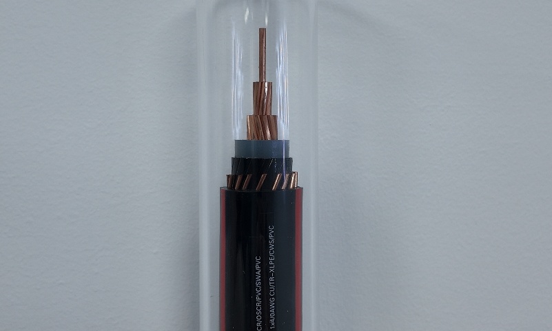
5-46kV TR-XLPE URD Medium Voltage Utility Cables
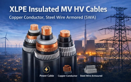
5–46kV TR-XLPE URD Medium Voltage Utility Power Cables are specifically designed for underground residential distribution and utility power networks. Manufactured with high-quality copper or aluminum conductors and tree-retardant cross-linked polyethylene (TR-XLPE) insulation, these cables provide superior resistance to electrical treeing, moisture ingress, and long-term aging. The TR-XLPE insulation system significantly extends service life in underground installations where environmental stress and moisture exposure are common. Rated for voltage levels from 5kV to 46kV, the cable ensures stable and efficient power transmission under continuous operating conditions. Its robust construction supports direct burial or duct installation, meeting the reliability requirements of modern utility infrastructure. Designed to meet utility and industry performance expectations, TR-XLPE URD cables offer consistent electrical performance, enhanced durability, and reduced maintenance over their operational lifespan.
10kV Cast Resin Dry Type Transformer Copper Winding
The 10kV Cast Resin Dry Type Transformer Copper Winding, a high-reliability, oil-free power solution engineered for safe and efficient indoor medium-voltage distribution. This three-phase dry-type transformer features fully vacuum-cast epoxy resin encapsulation around high-purity copper windings, combined with premium low-loss grain-oriented silicon steel cores to deliver exceptional energy efficiency (typically 98%+), significantly reduced no-load and load losses, and outstanding partial discharge performance (<10pC). The cast resin design ensures superior moisture resistance, self-extinguishing fire safety (F1 class), robust short-circuit withstand, and maintenance-free operation. Natural air (AN) cooling with optional forced air (AF) upgrades supports high overload capacity while maintaining low acoustic emissions through advanced vibration isolation and optimized core/winding geometry. Compliant with IEC 60076-11 and equivalent standards, this transformer steps down 10kV primary (with ±2×2.5% or wider off-circuit taps) to 0.4kV secondary (Dyn11 vector group standard), making it the ideal choice for modern commercial, industrial, and utility indoor installations prioritizing safety, sustainability, and long-term performance.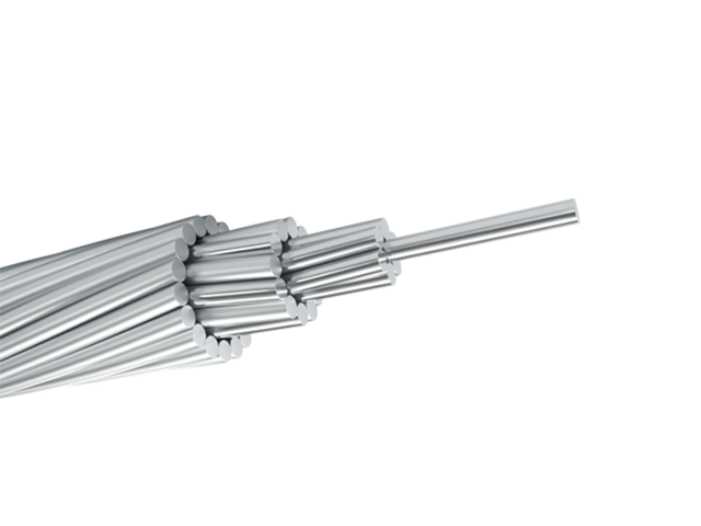
ACAR Conductor IEC 61089 Standard (A1/A3 & A1/A2) - Aluminum Alloy Reinforced
The ACAR Conductor IEC 61089 Standard (A1/A3, A1/A2) is a premium Aluminum Conductor Alloy Reinforced designed for efficient overhead power transmission and distribution. It consists of concentrically stranded 1350-H19 aluminum wires around a high-strength 6201-T81 aluminum-magnesium-silicon alloy core, offering an excellent balance of electrical conductivity and mechanical strength. Compared to equivalent ACSR conductors, this IEC 61089 ACAR provides higher ampacity at the same weight, lower sag, and superior corrosion resistance without steel core issues. Available in A1/A3 and A1/A2 configurations, it meets stringent IEC 61089 requirements for long-span lines. The ACAR Conductor IEC 61089 undergoes rigorous quality testing from raw materials to finished product, ensuring low DC resistance, high breaking strength, and reliable performance in various climates. Ideal for new installations or reconductoring projects where optimized strength-to-weight ratio and cost-effectiveness are critical.Welcome your inquiry
Honesty, Integrity, Frugality, Activeness and Passion